Local Clustering

Consider two scenarios of friendships:

First case:

Tom knows Susan, Tom knows Frank, Susan knows Frank, Frank knows Bob, Susan knows Bob, Tom knows Bob

In other words:

Tom is connected to Susan, Frank, and Bob
Susan and Frank are connected
Frank and Bob are connected
Susan and Bob are connected

If we focus only on Tom’s neighbourhood (i.e., the nodes Tom is directly connected to: Susan, Frank, Bob), we ask:

How interconnected are Susan, Frank, and Bob among themselves?

Susan ↔ Frank (yes)
Susan ↔ Bob (yes)
Frank ↔ Bob (yes)

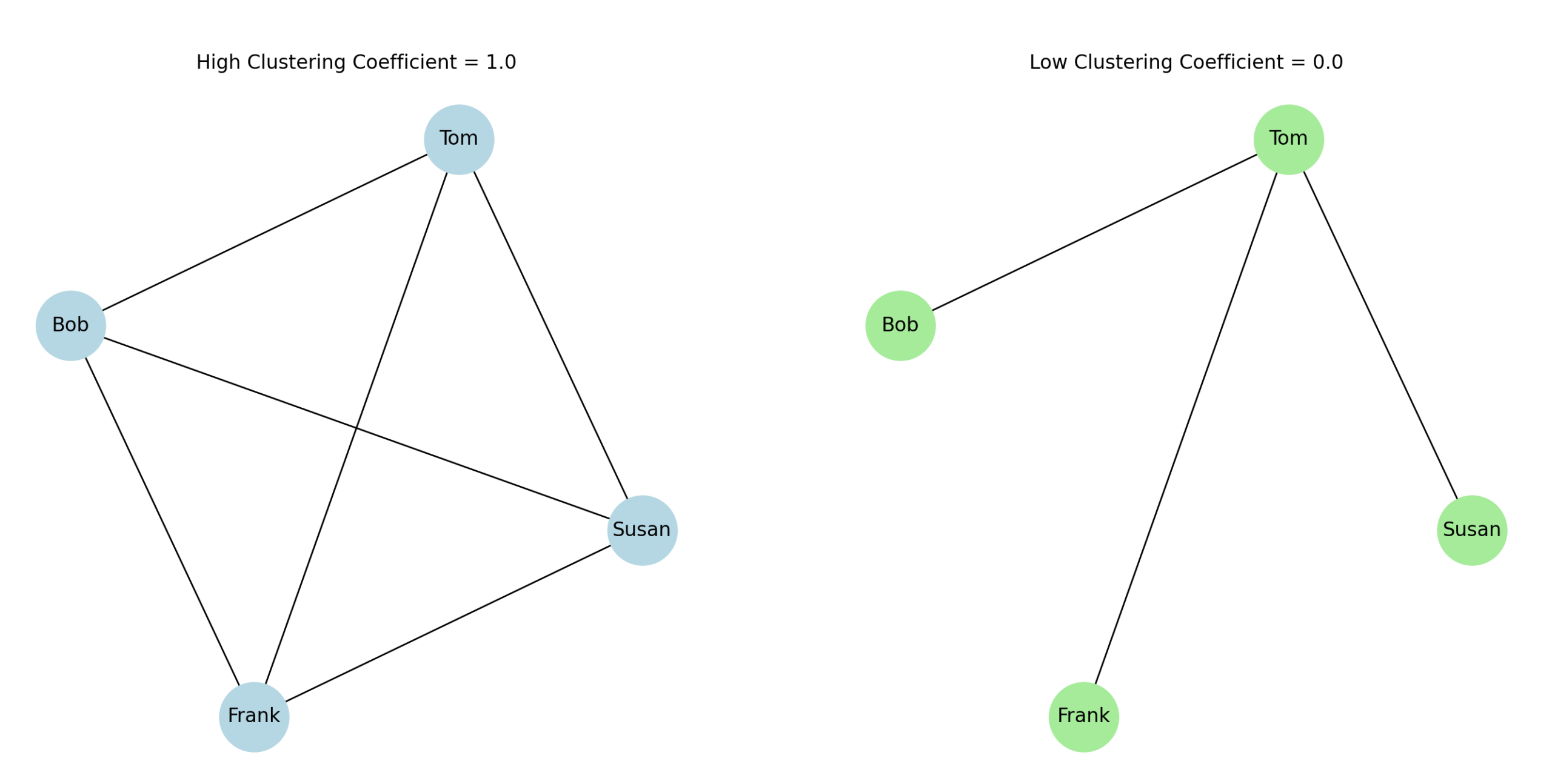
All three neighbours are fully connected among themselves, they form a triangle, all possible edges among Tom’s neighbours exist.

Maximal connections among neighbours → high clustering coefficient = 1.0

Now let’s consider another scenario:

Second case:

Tom knows Susan, Tom knows Frank, Tom knows Bob (no other connections)

Tom’s neighbourhood: Susan, Frank, Bob

Connections within Tom’s neighbourhood:

Susan ↔ Frank (no)
Susan ↔ Bob (no)
Frank ↔ Bob (no)

None of Tom’s neighbours are connected to each other.

Zero connections among neighbours → low clustering coefficient = 0.0

In the first scenario, Tom’s neighbours form many connections among themselves → high clustering coefficient. In the second scenario, Tom’s neighbours aren’t connected to each other → low clustering coefficient. Essentially, clustering coefficients measure how close a node’s neighbourhood is to forming a complete graph (clique).

So in mathematical terms, for a node $v$ with $d(v)$ neighbours, the local clustering coefficient $C_v$ measures the proportion of existing edges between neighbours to the total possible number of such edges:

$C_v = \frac{2T_v}{d(v)(d(v)-1)}$

where $T_v$ is the number of triangles containing node $v$ .

In the first scenario, Tom’s three neighbours (Susan, Frank, Bob) are all connected to each other, forming a complete triangle: $T_v$ = 3, yielding $C_v$ = 1.0. In the second scenario, none of Tom’s neighbours are connected: $T_v$ = 0, yielding $C_v$ = 0.0.

We can show this diagrammatically using the following python code:

import networkx as nx
import matplotlib.pyplot as plt

# First graph: high clustering (everyone connected)
G_high = nx.Graph()
G_high.add_edges_from([
    ("Tom", "Susan"), ("Tom", "Frank"), ("Tom", "Bob"),
    ("Susan", "Frank"), ("Susan", "Bob"), ("Frank", "Bob")
])

# Second graph: low clustering (only Tom connected)
G_low = nx.Graph()
G_low.add_edges_from([
    ("Tom", "Susan"), ("Tom", "Frank"), ("Tom", "Bob")
])

# Use same layout for both graphs
pos = nx.spring_layout(G_high, seed=42)

# Plot both graphs side by side
fig, axs = plt.subplots(1, 2, figsize=(12, 6))

# High clustering plot
nx.draw_networkx(G_high, pos=pos, ax=axs[0], with_labels=True, node_color='lightblue', edge_color='black', node_size=1800)
axs[0].set_title("High Clustering Coefficient = 1.0")

# Low clustering plot
nx.draw_networkx(G_low, pos=pos, ax=axs[1], with_labels=True, node_color='lightgreen', edge_color='black', node_size=1800)
axs[1].set_title("Low Clustering Coefficient = 0.0")

for ax in axs:
    ax.axis('off')

plt.show()

Which gives us:

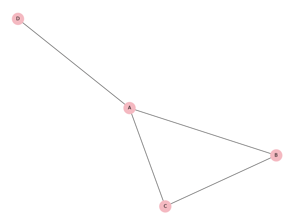
These are, of course, two extreme cases, maximal and minimal. In many scenarios, clustering coefficients are more nuanced. For example, consider a biological network where nodes represent proteins and edges represent physical interactions. Suppose protein A interacts with proteins B, C, and D. Among B, C, and D, only B and C interact with each other; D does not interact with either B or C.

Here, protein A’s neighbourhood consists of B, C, and D. There are 3 possible interactions among A’s neighbours: B–C, B–D, and C–D. Only 1 of these 3 interactions exists (the interaction between B and C). Therefore, the clustering coefficient for protein A is:

$C_A = \frac{2T_A}{d(A)(d(A)-1)} = \frac{2 \times 1}{3 \times 2} = \frac{2}{6}$ = 0.333

This intermediate value reflects that some, but not all, of A’s interaction partners are themselves interconnected. Such partial clustering is typical in biological networks, where certain proteins form tightly connected complexes, while others bridge between more distant functional groups.

Again, let’s generate a graph diagram using python:

import networkx as nx
import matplotlib.pyplot as plt

# Create the graph
G = nx.Graph()

# Add edges
G.add_edges_from([
    ("A", "B"),  # Protein A interacts with B
    ("A", "C"),  # Protein A interacts with C
    ("A", "D"),  # Protein A interacts with D
    ("B", "C")   # B and C interact
    # No edge between B-D or C-D
])

# Define layout
pos = nx.spring_layout(G, seed=42)

# Draw the graph
plt.figure(figsize=(8, 6))
nx.draw_networkx(G, pos, with_labels=True, node_color='lightpink', edge_color='black', node_size=900)

# Remove axis
plt.axis('off')

plt.show()

Which plots:

Fig 2. Partial clustering, $C_A$ = 0.333

Local clustering variance

We’ve said that local clustering coefficients measure how interconnected each node’s immediate neighbours are. But this value doesn’t stay the same across all nodes in a network, it can vary widely depending on the node’s role and position. For example, nodes that belong to tightly knit groups or cliques tend to have high local clustering coefficients, because most of their neighbours are also connected to each other. This is typical in social groups, protein complexes, or communities where everyone interacts frequently. In contrast, nodes that act as bridges or hubs connecting different parts of the network often have lower local clustering coefficients. Even though they might have many connections (high degree), their neighbours are not necessarily connected to each other. Think of a company CEO connecting different departments, or a protein linking multiple functional modules.

Local clustering can indicate social redundancy or resilience

A high local clustering coefficient means that a node’s neighbours are tightly connected. This can imply redundancy of connections: if the node were removed, its neighbours would still be linked via each other. In social networks, this suggests robustness of communication inside a clique. In biological networks, it may imply functional redundancy (e.g., backup pathways in metabolism). In contrast, a low clustering node is often more structurally vulnerable, its removal might disconnect otherwise distant nodes.

Local clustering correlates with different roles in the network

High clustering nodes are often peripheral or modular nodes, embedded within a specific community. Low clustering nodes are often brokers, bridges, or hubs connecting multiple communities. This makes local clustering complementary to measures like betweenness centrality, they describe whether a node is a community core or a connector between groups.

Local clustering is influenced by degree

In many real-world networks (especially scale-free networks), nodes with higher degree tend to have lower clustering coefficients on average. Why? Because it’s harder for all the neighbours of a highly connected node to also be connected to each other. This is known as a degree–clustering relationship, it reflects hierarchical or hub-like structure. In contrast, nodes with low degree can more easily form complete triangles.

Local clustering can be used to identify overlapping communities or functional modules

Nodes with similar clustering coefficients often belong to the same structural type:

High clustering nodes → interior of communities
Medium clustering → boundary nodes
Low clustering → inter-community bridges

This makes clustering useful for detecting overlapping or fuzzy community boundaries.

Interpretation depends on the network type

Social networks: high clustering → tight friend groups
Biological networks: high clustering → protein complexes, regulatory modules
Technological networks: high clustering → redundant circuits or backup routes

So the same numerical value has different interpretations across domains.